Theoretical aspects

Tiles

The goal of this section is to describe how the tiles behave geometrically through specifying their Origin, dimensions and Euler angles.

In general, the demagnetization tensor for each tile type is found with respect to the local Origin of the tile and assuming the tile not to be rotated. The tile’s local Origin is defined through the vector \(r'\) with respect to the global Origin. The field is found at the position \(r\) with respect to the global coordinate system (G).

We let P denote the matrix representing the mapping from the local (L) to the global coordinate system (G). As the demagnetization tensor is always found with respect to L and it takes the relative distance as input, we get the geometrical part of the field (not including magnetization) to be:

\[K(r) = \text{P} N (\text{P}^{-1}(r - r')).\]

The magnetization with respect to the global coordinate system is given by (for a hard magnet characterized by an anisotropic permeability tensor):

\[[M]_G = (\text{P}[\mu]_L) H + M_{rem}[\hat{u}_{ea}]_G,\]

where the magnetic field in the global system is denoted \(H\), the magnitude of the remanence is \(M_{rem}\) and the unit vector defining the easy-axis of the permanent magnet in the global system is \([\hat{u}_{ea}]_G = \text{P} [\hat{u}_{ea}]_L\). As an example, consider e.g. a prism magnetized along the prism’s x-direction. Then \([\hat{u}_{ea}]_L = (1, 0, 0)\).

The field in the global system then becomes:

\[\begin{split}H &= K(r)[M]_L = K(r) \text{P}^{-1} [M]_G \\ & = \text{P} N (\text{P}^{-1}(r - r')) (\text{P}[\mu]_L) H + \text{P} (M_{rem}[\hat{u}_{ea}]_L)\end{split}\]

Now, finding the P matrix and its inverse needs to be done. This is described in the section rotations.

Rotations

So far, we only consider this transformation to consist of three rotations; about the \(x\), \(y\) and \(z\) axes in that order with the angles \(\phi\) (roll), \(\theta\) (pitch) and \(\psi\) (yaw). Since the global coordinate system coincides with the canonical xyz-system, P simply consists of the three (column) vectors defining the orthonormal basis of the local system, expressed with respect to the global system:

\[\text{P} = \{ [\hat{e_x}]^T_G, [\hat{e_y}]^T_G, [\hat{e_z}]^T_G \}\]

These unit vectors may be found through applying the rotation matrices in the correct order (intrinsic rotation with sequence \(x_L-y_L'-z_L''\) or extrinsic rotations with \(z_G-y_G-x_G\)):

\[\text{P} = Rot_x(\phi) Rot_y(\theta) Rot_z(\psi).\]

Finally, as P is orthogonal, we have that

\[\begin{split}\text{P}^{-1} &= Rot_z(\psi)^{-1} Rot_y(\theta)^{-1} Rot_x(\phi)^{-1} \\ & = Rot_z(\psi)^T Rot_y(\theta)^T Rot_x(\phi)^T\end{split}\]

Implementation

In the code, the rotation matrix rotMat and its inverse rotMatInv are calculated. They are applied in the subroutine getFieldFromTile. Hereby, the evaluation points, which are defined with respect to the global coordinate system, are rotated with rotMat into the local system of the considered tile.

The three rotation angles (\(\phi, \theta, \psi\)) rotate the given tile intrinsically about the orthonormal basis of the local system in the order \(x_L-y_L'-z_L''\). This corresponds to a extrinsic rotation with sequence \(z_G-y_G-x_G\) in the global system.

To bring the evaluation points into the local system of the considered tile, the negative rotation angles have to be applied in opposite order.

\[\begin{split}Rot_x(-\phi) = \begin{bmatrix} 1 & 0 & 0\\ 0 & cos(-\phi) & -sin(-\phi)\\ 0 & sin(-\phi) & cos(-\phi) \end{bmatrix} = \begin{bmatrix} 1 & 0 & 0\\ 0 & cos(\phi) & sin(\phi)\\ 0 & -sin(\phi) & cos(\phi) \end{bmatrix} = Rot_x(\phi)^T.\end{split}\]

Similarly, \(Rot_y(-\theta) = Rot_y(\theta)^T\) and \(Rot_z(-\psi) = Rot_z(\psi)^T\).

rotMat and rotMatInv are defined as follows:

\[\begin{split}\text{rotMat} &= Rot_z(-\psi) Rot_y(-\theta) Rot_x(-\phi) \\ & = Rot_z(\phi)^T Rot_y(\theta)^T Rot_x(\psi)^T\end{split}\]

\[\begin{split}\text{rotMatInv} &= Rot_x(-\phi)^T Rot_y(-\theta)^T Rot_z(-\psi)^T \\ & = Rot_x(\phi) Rot_y(\theta) Rot_z(\psi)\end{split}\]

rotMatInv is the mapping from the local system of the given tile to the global coordinate system and corresponds to our P in the theoretical part. As we are performing a rotation in the local system (intrinsically), post-multiplication applies for the rotation matrices.

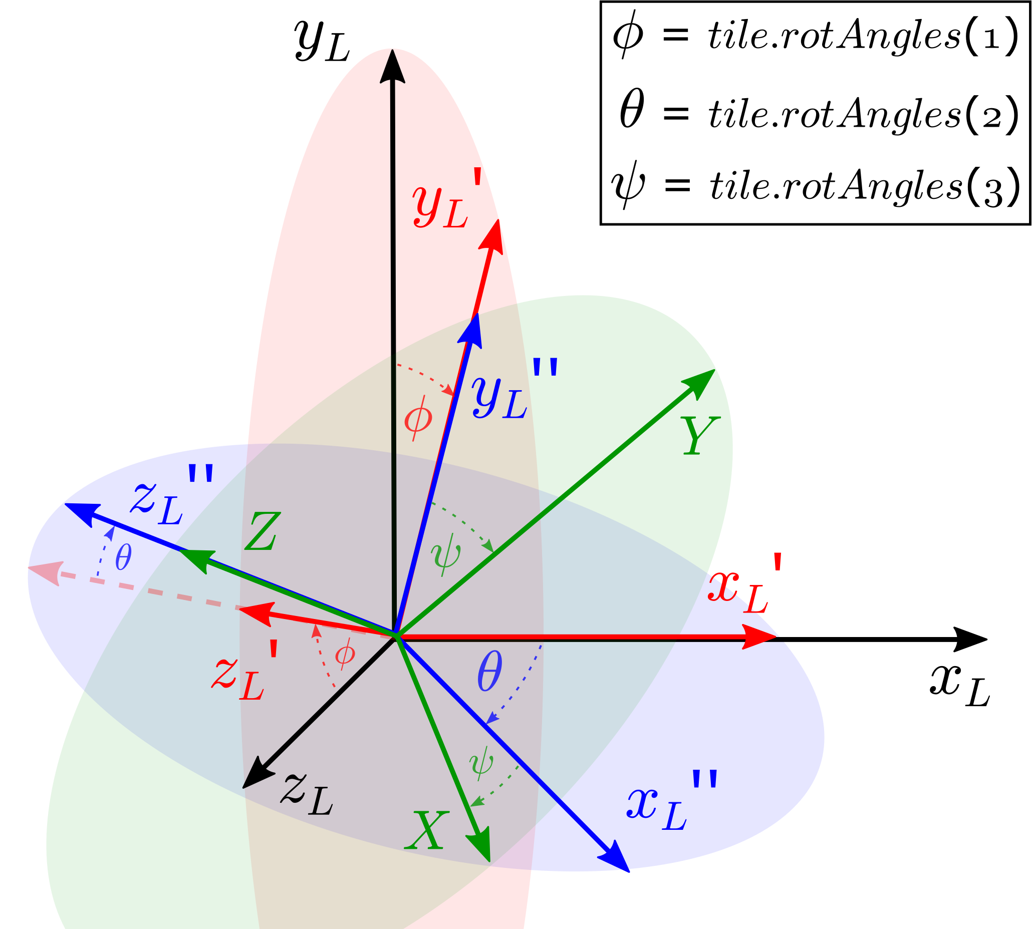
Rotations of a tile are performed in its local coordinate system. Firstly, the tile is rotated with \(\phi\) around its local x-axis. Secondly, the local y-axis is rotated by \(\theta\). Eventually, the angle \(\psi\) is performed around the local z-axis. \(\{ X^T, Y^T, Z^T\} \hat{=} \{ [\hat{e_x}]^T_G, [\hat{e_y}]^T_G, [\hat{e_z}]^T_G \}\).